Laplace Transform Techniques in Circuit Analysis

Laplace Transforms of Important Functions

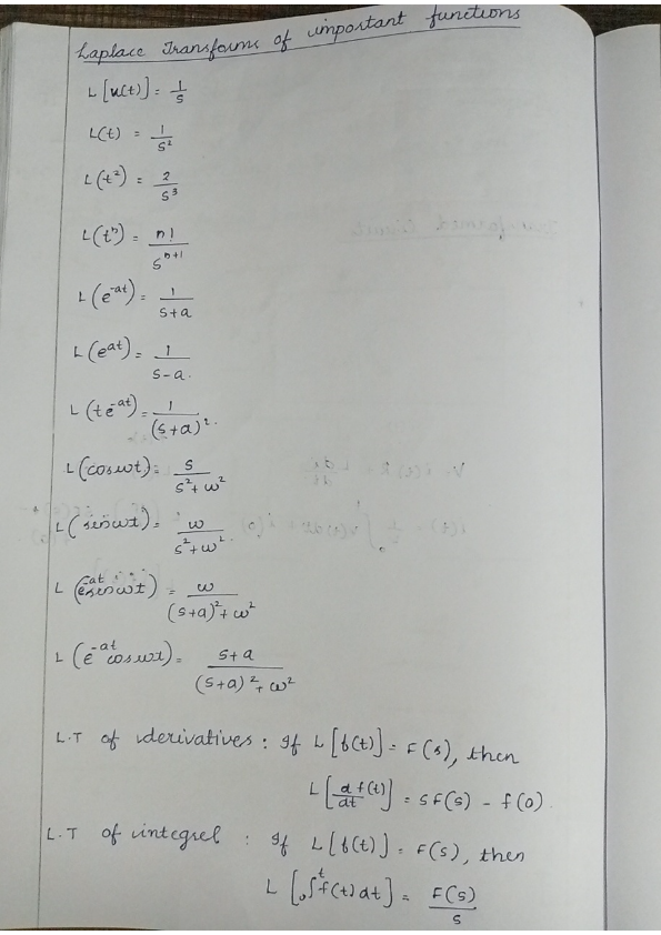
Basic Laplace Transforms

1. Unit Step Function: $L[u(t)] = \frac{1}{s}$

   • The unit step function is often used to model systems that switch on at a specific time.

2. Constant Function: $L(t) = \frac{1}{s^2}$

   • Represents a constant rate or acceleration in a system.

3. Polynomial Functions: $L(t^2) = \frac{2}{s^3}$

   • General form: $L(t^n) = \frac{n!}{s^{n+1}}$
   • Useful for analyzing free response of systems and solving differential equations involving polynomials.

4. Exponential Decay: $L(e^{-at}) = \frac{1}{s+a}$

   • Models processes like radioactive decay and cooling.

5. Exponential Growth: $L(e^{at}) = \frac{1}{s-a}$

   • Used in contexts like population growth or compounding interest.

6. Exponential Times Polynomial: $L(t e^{-at}) = \frac{1}{(s+a)^2}$

   • Useful in more complex system responses involving time-delay effects.

Trigonometric Functions

1. Cosine Function: $L(\cos \omega t) = \frac{s}{s^2 + \omega^2}$

   • Describes oscillatory systems, such as electrical circuits or mechanical vibrations.

2. Sine Function: $L(\sin \omega t) = \frac{\omega}{s^2 + \omega^2}$

   • Similar applications to cosine, often used with initial conditions.

3. Damped Sine Wave: $L(e^{-at} \sin \omega t) = \frac{\omega}{(s+a)^2 + \omega^2}$

   • Models systems where oscillation amplitude decreases over time, like shock absorbers.

4. Damped Cosine Wave: $L(e^{-at} \cos \omega t) = \frac{s+a}{(s+a)^2 + \omega^2}$

   • Applies to damped oscillatory systems.

Derivatives and Integrals

• Derivatives:

  • If $L[f(t)] = F(s)$, then: $L\left[\frac{d}{dt}f(t)\right] = sF(s) - f(0)$
  • The derivative formula links the time domain to the s-domain by introducing a multiplicative factor $s$ and accounting for initial conditions.

• Integrals:

  • If $L[f(t)] = F(s)$, then: $L\left[\int f(t) dt \right]= \frac{F(s)}{s}$
  • Integration in the Laplace domain corresponds to division by $s$, useful for solving differential equations with integral terms.

These Laplace transform relationships are essential tools for engineers and scientists to analyze and solve linear time-invariant systems, especially in control systems, signal processing, and differential equations. They simplify the handling of complex systems by converting differential equations into algebraic ones.

Extended readings:

Transformed Circuits

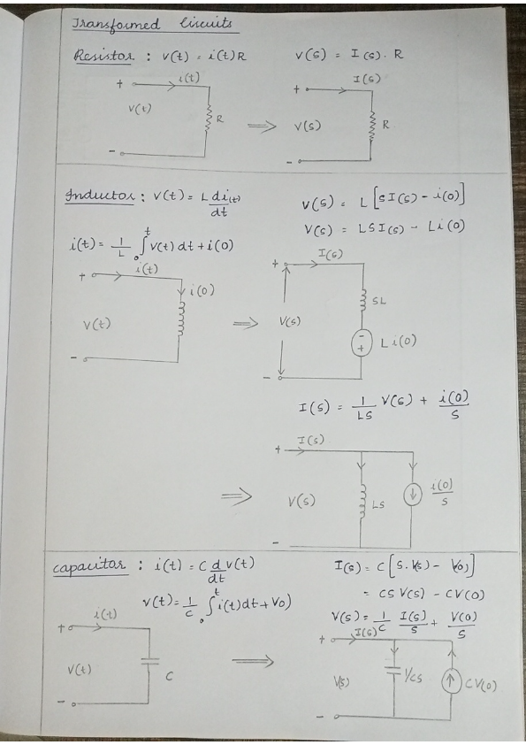
Resistor

• Equation: $V(t) = i(t)R$

  • A resistor follows Ohm's Law, where the voltage across the resistor is directly proportional to the current through it, multiplied by its resistance $R$.

• Laplace Transform: $V(s) = I(s) \cdot R$

  • In the Laplace domain, the transformation simplifies the analysis of linear time-invariant systems. The impedance of a resistor remains $R$.

• Circuit Representation:

  • Original: A simple resistor with input voltage $V(t)$ and current $i(t)$.
  • Transformed: Resistor with impedance $R$ and input current $I(s)$.

Inductor

• Equation: $V(t) = L \frac{di(t)}{dt}$

  • The voltage across an inductor is proportional to the rate of change of current through it, scaled by inductance $L$.

• Laplace Transform:

  • $V(s) = L[sI(s) - i(0)]$
  • $I(s) = \frac{1}{Ls} V(s) + \frac{i(0)}{s}$
  • These transformations account for the initial current $i(0)$, showing how the inductance's stored energy affects current and voltage over time.

• Circuit Representation:

  • Original: An inductor with initial current $i(0)$.
  • Transformed: Inductor $Ls$ in series with a voltage source $L \cdot i(0)$.

Capacitor

• Equation: $i(t) = C \frac{dV(t)}{dt}$

  • The current through a capacitor is proportional to the rate of change of voltage across it, determined by the capacitance $C$.

• Laplace Transform:

  • $I(s) = C[sV(s) - V(0)]$
  • $V(s) = \frac{1}{Cs} I(s) + \frac{V(0)}{s}$
  • These equations highlight how a capacitor initially charged to $V(0)$ affects system behavior in the Laplace domain.

• Circuit Representation:

  • Original: A capacitor with initial voltage $V(0)$.
  • Transformed: Capacitor $\frac{1}{Cs}$ in parallel with a voltage source $\frac{V(0)}{s}$.

Insights:

• Laplace Transformation: A mathematical tool used to convert differential equations into algebraic equations, making complex systems easier to handle, especially for control systems and signal processing.

• Impedance in s-domain: For analysis in the Laplace domain, resistors, inductors, and capacitors are treated with their respective impedances $R$, $sL$, and $\frac{1}{sC}$.

• Initial Conditions: When transforming to the $s$-domain, initial conditions are crucial as they represent the stored energy in capacitors and inductors, influencing system response.

Extended readings:

LAPLACE CIRCUIT ANALYSIS NOTES

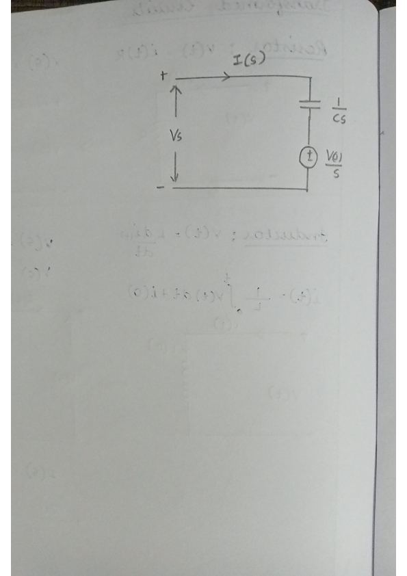
Circuit Diagram

Description

• Components:
  • Current Source: $V_0/s$.
  • Capacitor: $\frac{1}{Cs}$.
  • Voltage Source: $V_s$.
• Current: $I(s)$.

Insights

• Laplace Transform: The use of $V(s)$ and $I(s)$ indicates the application of Laplace transforms to circuit analysis, a powerful method to handle circuits in the s-domain.
• Complex Frequency: The variable $s$ represents complex frequency, $s = \sigma + j\omega$, where $\sigma$ is the growth rate and $j\omega$ is the oscillation.

Additional Concepts

Capacitive Reactance

• Reactance in S-Domain: $X_c(s) = \frac{1}{Cs}$
  • Represents how a capacitor behaves as an impedance in the s-domain, inversely proportional to both the capacitance $C$ and $s$.

Initial Conditions

• Initial Charge or Current:
  • The term $\frac{V_0}{s}$ suggests an initial voltage, which is transformed from the time domain to the s-domain, accommodating initial conditions directly in Laplace analysis.

Analysis Strategy

• Use Kirchhoff’s laws in the s-domain to set up equations involving voltage and current.
• Solve algebraically for desired quantities, such as node voltages or branch currents, using known transforms.
• Convert back to the time domain using inverse Laplace transform, if necessary.

Example Application

1. Find $I(s)$ in terms of known quantities:

   • Write the equation using KVL or KCL in the $s$ domain.
   • Example: $V_s = I(s) \cdot \frac{1}{Cs} + \frac{V_0}{s}$
   • Solve for $I(s)$.

2. Time-Domain Analysis:

   • Use inverse Laplace transform to revert known quantities back to the time domain.
   • Apply initial conditions where applicable to determine specific solutions in physical time.

General Tips

• Make sure to account for all initial conditions due to their impact on the s-domain equations.
• Familiarize yourself with standard Laplace transforms and their inverses, as they simplify solving differential equations.

Extended readings: